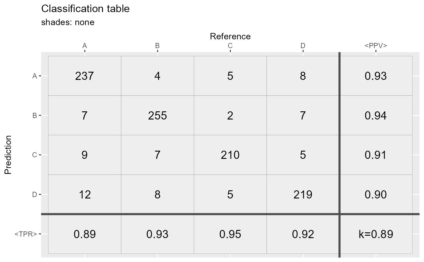
[!+] Plot a confusion matrix (a.k.a. classification table)

Plot a confusion matrix (classification table) with additional statistics (sensitivity (Se) a.k.a. true positive rate, positive predictive value (PPV) and Cohens' Kappa (k)).

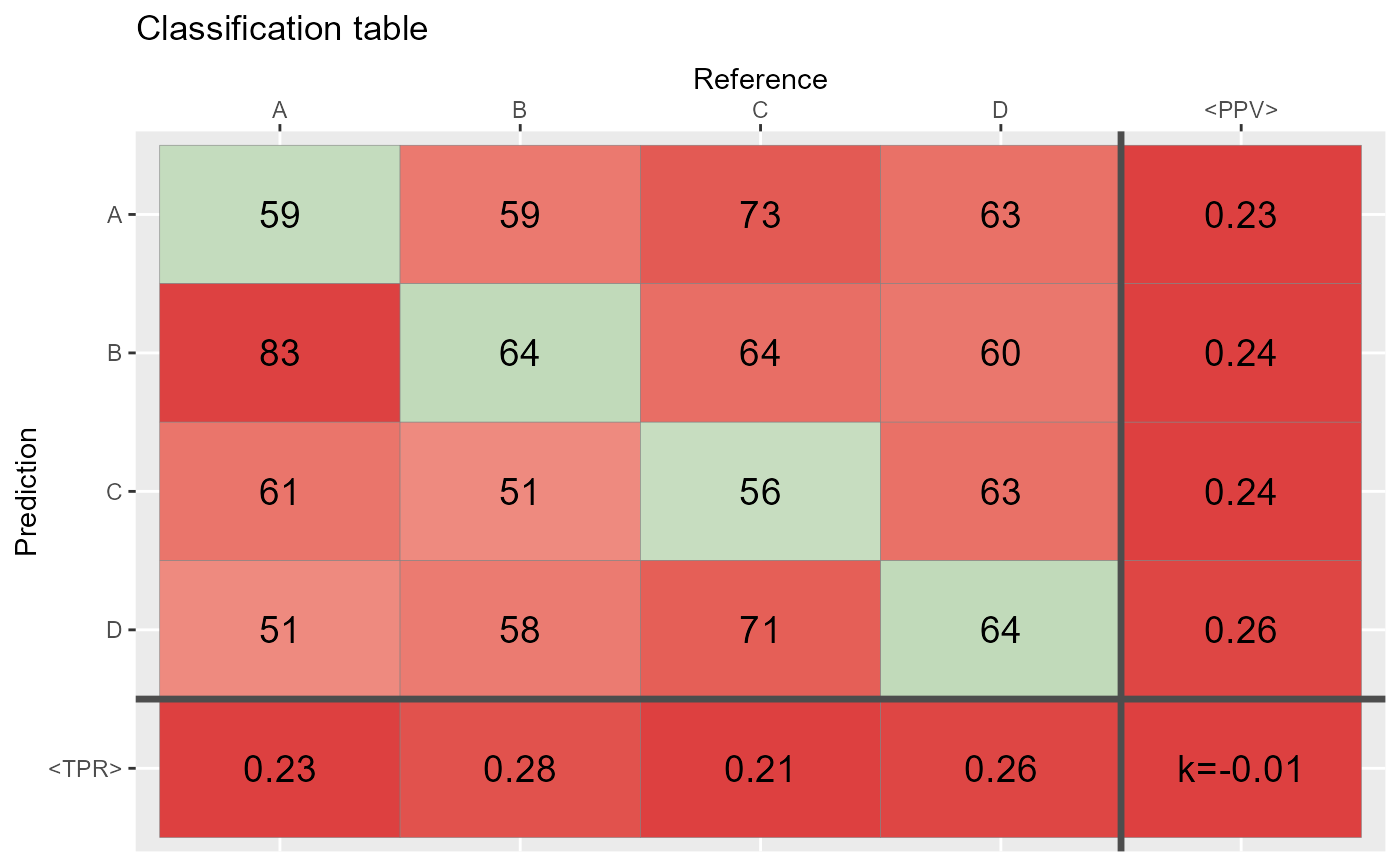
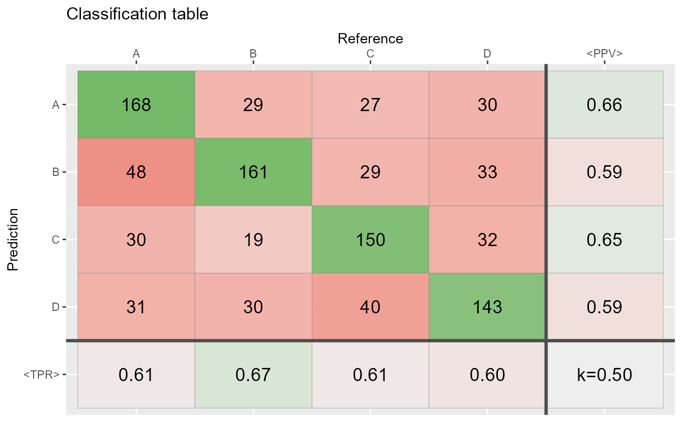
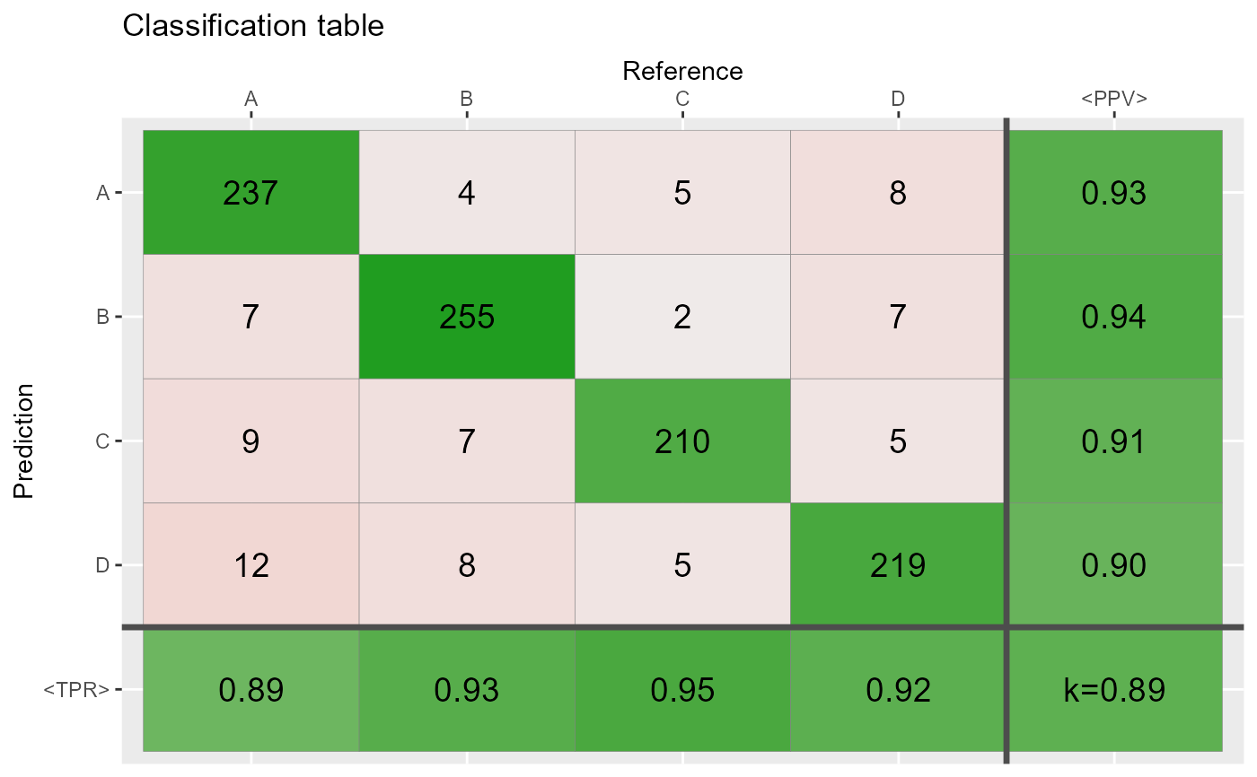
Colors in the main matrix: diagonal cells vary from grey to green and offdiagonal elements vary from grey to red. The color intensity in certain cell is determined by parameter shades.

Colors of cells with statistics Se, PPV and k vary depening on values of these statistics from red (low values) to grey (middle values), to green (high values).

Exception: when shades="const" and shades="none", color intensities are constant.

qplot_confusion(...)

# S3 method for default
qplot_confusion(
  Prediction,
  Reference,
  Title = "Classification table",
  xLabel = NULL,
  yLabel = NULL,
  subTitle = NULL,
  shades = c("prop", "max", "const", "none"),
  guide = FALSE,
  text.size = 5,
  decimals = 2,
  ...
)

# S3 method for matrix
qplot_confusion(mat, ...)

# S3 method for ResampleResult
qplot_confusion(obj, ...)

# S3 method for PredictionClassif
qplot_confusion(obj, ...)

# S3 method for table
qplot_confusion(
  conf,
  Title = "Classification table",
  xLabel = NULL,
  yLabel = NULL,
  subTitle = NULL,
  shades = c("prop", "max", "const", "none"),
  guide = FALSE,
  text.size = 5,
  decimals = 2,
  TPR.name = "<TPR>",
  PPV.name = "<PPV>",
  sort = c(FALSE, "diagonal", "PPV", "TPR"),
  metric = c("kappa", "weighted.kappa", "meanTPR", "meanPPV")
)

Arguments

...

Appropriate parameters (described below).

Prediction

A factor variable with predicted groups.

Reference

A factor variable with reference groups.

Title

The main title for the plot.

xLabel

A label for abscisa (x) axis.

yLabel

A label for ordinate (y) axis.

subTitle

The second line of title, which will be smaller and and in italics.

shades

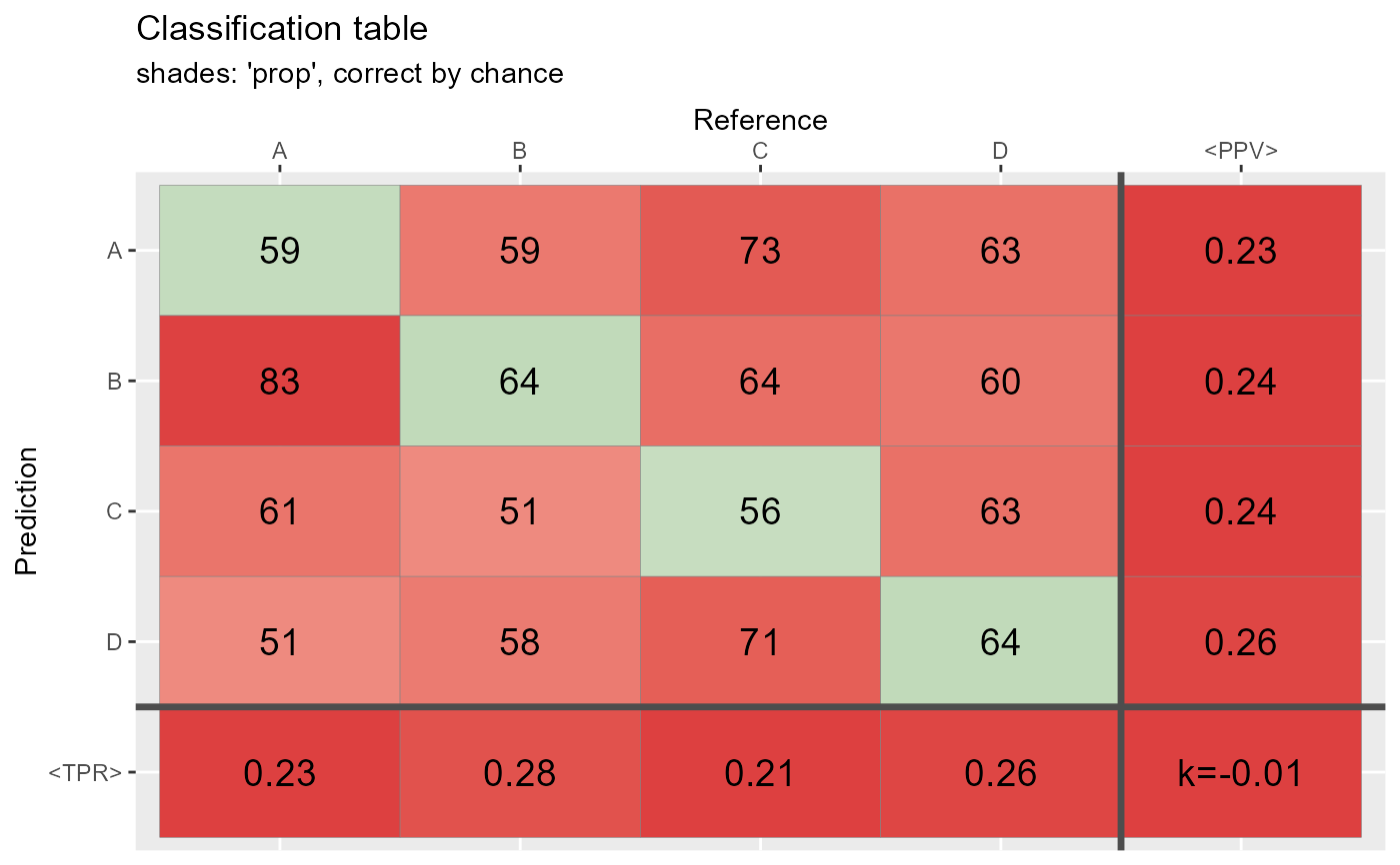
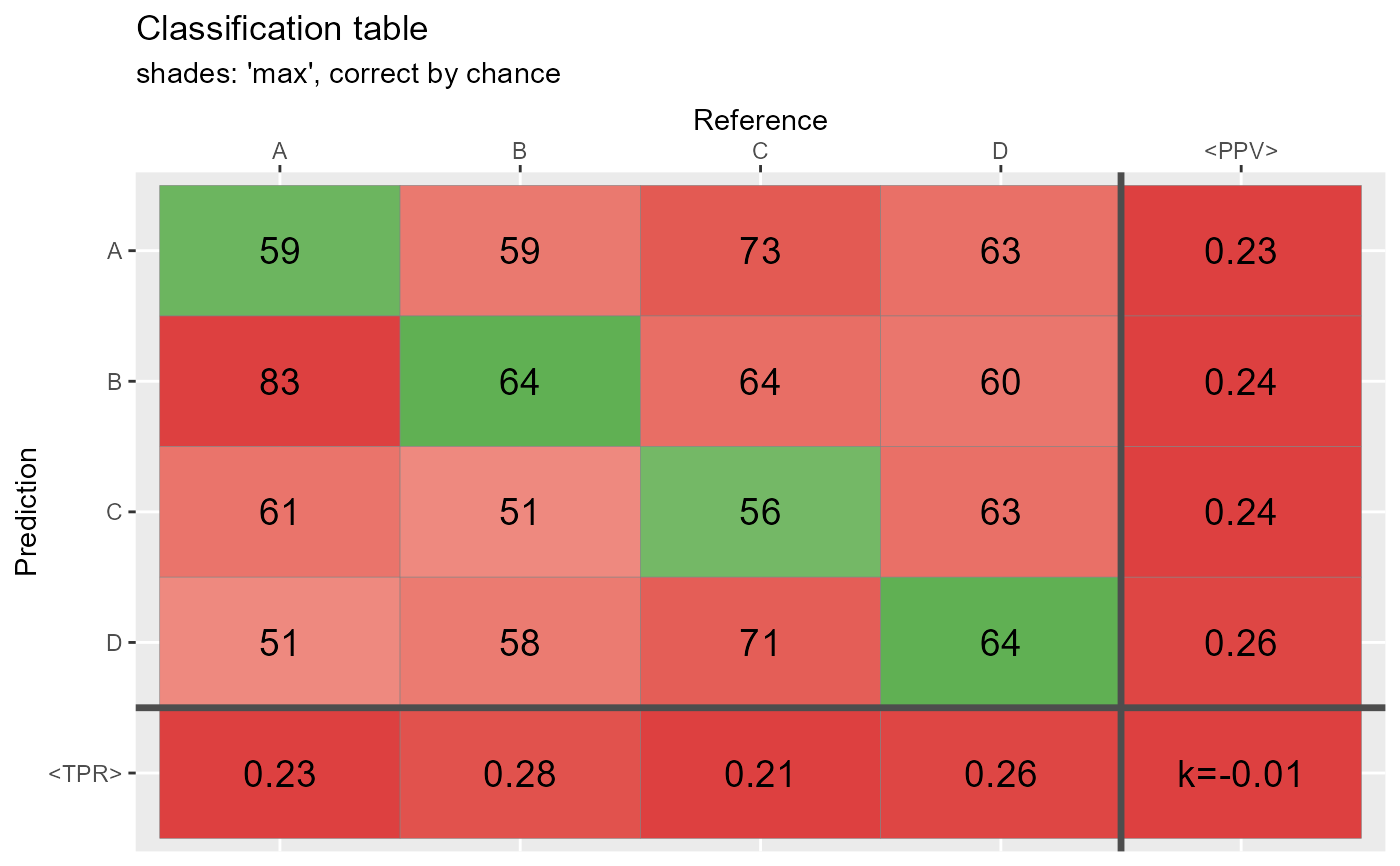
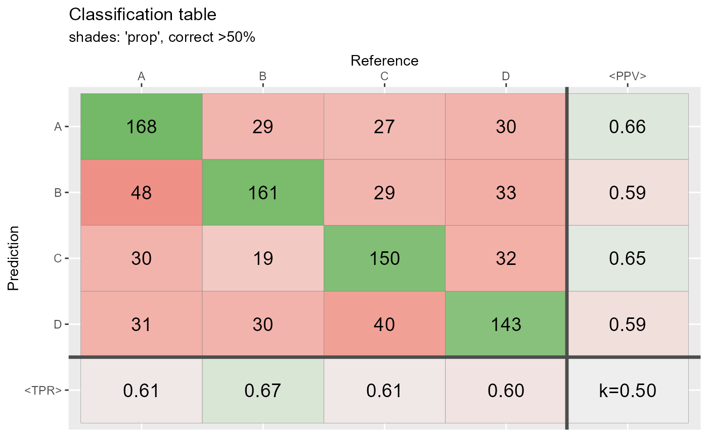
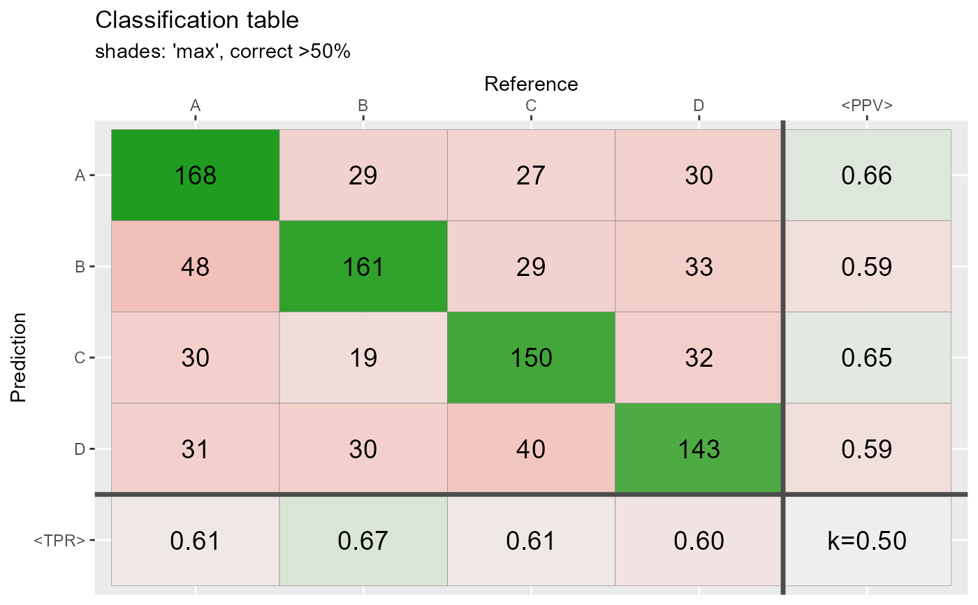
A function how intensities of cell colors in the main confsion matrix depend on cell values:

"prop"

An intensity of a cell color is proportianal to a value in the cell. Distribution of color intensities is balanced according to number of classes (but not balanced according to number of observations per class.)

"max"

Cell with the absolute maximum value is represented by the most intensive color. Other cells are proportionally less intensive.

"const"

Constant red and green colors.

"none"

All cells are grey.

guide

Logical. If TRUE, a legend is plotted.

text.size

The size of a text inside cells.

decimals

The number of decimal positions in rounding. Default is 2 (i.e., precission is 0.01).

conf, mat

A confusion matrix (classification table): either an object of a class "table" or a square matrix.

TPR.name

The name of the row with true positive rate (TPR). Default is "<TPR>". It is the same as "<Sensitivity>".

PPV.name

The name of the column with positive predictive value (PPV). Default is "<PPV>".

sort

A way to sort columns and rows of output matrix. Options to sort values in descending order:
FALSE (default) do not sort;
"diagonal" - sort values on diagonal;
"PPV" - sort positive predictive values (PPV);
"TPR" - sort true positive rate (TPR) values.

metric

The metric of overall accuracy. Curently supported values are:
"kappa" (default) to use Cohen's kappa, in table denoted with symbol "k";
"weighted.kappa" to use weighted kappa, (symbol "w");
"meanTPR" Mean of true positive rates of each group (symbol "t");
"meanPPV" Mean of positive predictive values of each group (symbol "v").

Value

A plot of confusion matrix and additional statistics (`ggplot` object).

See also

Other spHelper plots: check_palette(), layer_spRangeMean(), plot_colors(), plot_hyPalette(), plot_spCompare(), plot_spDiff(), plot_spDistribution(), qplot_crosstab(), qplot_infoDim(), qplot_kAmp(), qplot_kSp(), qplot_prediction(), qplot_spRangeCenter(), qplot_spRangeMedian(), qplot_spStat(), qplot_spc(), rmExpr(), rm_stripes(), stat_chull()

Author

Vilmantas Gegzna

Examples

# Generate data: Random guess  ============================
 N <- 1000 # number of observations

Prediction <- sample(c("A","B","C","D"), N, replace = TRUE)
Reference  <- sample(c("A", "B","C","D"),N, replace = TRUE)

# This function:
qplot_confusion(Prediction, Reference)


# does the same as:
conf <- table(Prediction,Reference)
qplot_confusion(conf)


# At least 50% of the cases agree =========================
ind <- sample(1:N,round(0.50*N))
Reference[ind] <- Prediction[ind]
conf2 <- table(Prediction,Reference)

qplot_confusion(conf2)


# Most of the cases agree =================================
ind <- sample(1:N,round(N*.80))
Reference[ind] <- Prediction[ind]
conf3 <- table(Prediction,Reference)

qplot_confusion(conf3)


# Proportions =============================================

qplot_confusion(conf3)


# Shades: proportional =====================================

qplot_confusion(conf,shades = "prop",  subTitle = "shades: 'prop', correct by chance")

qplot_confusion(conf,shades = "max",   subTitle = "shades: 'max', correct by chance")


qplot_confusion(conf2,shades = "prop", subTitle = "shades: 'prop', correct >50%")

qplot_confusion(conf2,shades = "max",  subTitle = "shades: 'max', correct >50%")


qplot_confusion(conf3,shades = "prop", subTitle = "shades: 'prop', correct >80%")

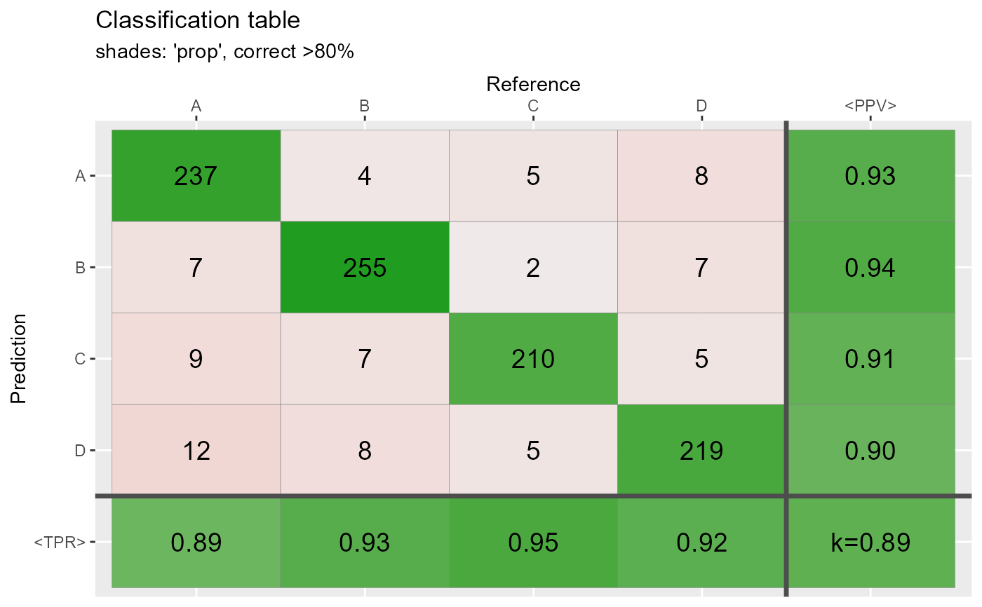qplot_confusion(conf3,shades = "max",  subTitle = "shades: 'max', correct >80%")


# Shades: constant and none ================================

qplot_confusion(conf3,shades = "const",subTitle = "shades: constant")

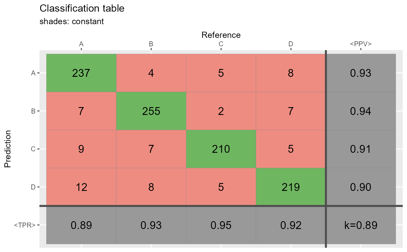qplot_confusion(conf3,shades = "none", subTitle = "shades: none")